The Scientist and Engineer's Guide to
Digital Signal Processing
By Steven W. Smith, Ph.D.

• Home
• The Book by Chapters
• About the Book
  • Copyright and permissible use
  • What is DSP?
  • 8 good reasons for learning DSP
  • Comments by reviewers
  • Errata
  • Free Software and Teaching Aids
  • Differences Between Editions
• Steven W. Smith
• Blog
• Contact

To start the discussion of recursive filters, imagine that you need to extract information from some signal, x[ ]. Your need is so great that you hire an old mathematics professor to process the data for you. The professor's task is to filter x[ ] to produce y[ ], which hopefully contains the information you are interested in. The professor begins his work of calculating each point in y[ ] according to some algorithm that is locked tightly in his over-developed brain. Part way through the task, a most unfortunate event occurs. The professor begins to babble about analytic singularities and fractional transforms, and other demons from a mathematician's nightmare. It is clear that the professor has lost his mind. You watch with anxiety as the professor, and your algorithm, are taken away by several men in white coats.

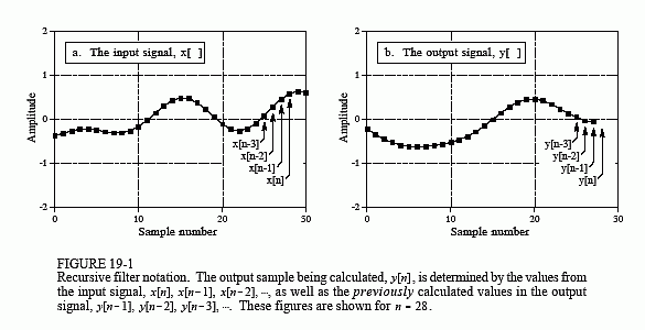
You frantically review the professor's notes to find the algorithm he was using. You find that he had completed the calculation of points y[0] through y[27], and was about to start on point y[28]. As shown in Fig. 19-1, we will let the variable, n, represent the point that is currently being calculated. This means that y[n] is sample 28 in the output signal, y[n - 1] is sample 27, y[n - 2] is sample 26, etc. Likewise, x[n] is point 28 in the input signal, x[n - 1] is point 27, etc. To understand the algorithm being used, we ask ourselves: "What information was available to the professor to calculate y[n], the sample currently being worked on?"

The most obvious source of information is the input signal, that is, the values: x[n], x[n - 1], x[n - 2], …. The professor could have been multiplying each point in the input signal by a coefficient, and adding the products together:

You should recognize that this is nothing more than simple convolution, with the coefficients: a₀, a₁, a₂, …, forming the convolution kernel. If this was all the professor was doing, there wouldn't be much need for this story, or this chapter. However, there is another source of information that the professor had access to: the previously calculated values of the output signal, held in: y[n - 1], y[n - 2], y[n - 3], …. Using this additional information, the algorithm would be in the form:

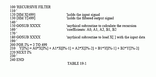
In words, each point in the output signal is found by multiplying the values from the input signal by the "a" coefficients, multiplying the previously calculated values from the output signal by the "b" coefficients, and adding the products together. Notice that there isn't a value for b₀, because this corresponds to the sample being calculated. Equation 19-1 is called the recursion equation, and filters that use it are called recursive filters. The "a" and "b" values that define the filter are called the recursion coefficients. In actual practice, no more than about a dozen recursion coefficients can be used or the filter becomes unstable (i.e., the output continually increases or oscillates). Table 19-1 shows an example recursive filter program.

Recursive filters are useful because they bypass a longer convolution. For instance, consider what happens when a delta function is passed through a recursive filter. The output is the filter's impulse response, and will typically be a sinusoidal oscillation that exponentially decays. Since this impulse response in infinitely long, recursive filters are often called infinite impulse response (IIR) filters. In effect, recursive filters convolve the input signal with a very long filter kernel, although only a few coefficients are involved.

The relationship between the recursion coefficients and the filter's response is given by a mathematical technique called the z-transform, the topic of Chapter 31. For example, the z-transform can be used for such tasks as: converting between the recursion coefficients and the frequency response, combining cascaded and parallel stages into a single filter, designing recursive systems that mimic analog filters, etc. Unfortunately, the z-transform is very mathematical, and more complicated than most DSP users are willing to deal with. This is the realm of those that specialize in DSP.

There are three ways to find the recursion coefficients without having to understand the z-transform. First, this chapter provides design equations for several types of simple recursive filters. Second, Chapter 20 provides a "cookbook" computer program for designing the more sophisticated Chebyshev low-pass and high-pass filters. Third, Chapter 26 describes an iterative method for designing recursive filters with an arbitrary frequency response.