The Scientist and Engineer's Guide to
Digital Signal Processing
By Steven W. Smith, Ph.D.

• Home
• The Book by Chapters
• About the Book
  • Copyright and permissible use
  • What is DSP?
  • 8 good reasons for learning DSP
  • Comments by reviewers
  • Errata
  • Free Software and Teaching Aids
  • Differences Between Editions
• Steven W. Smith
• Blog
• Contact

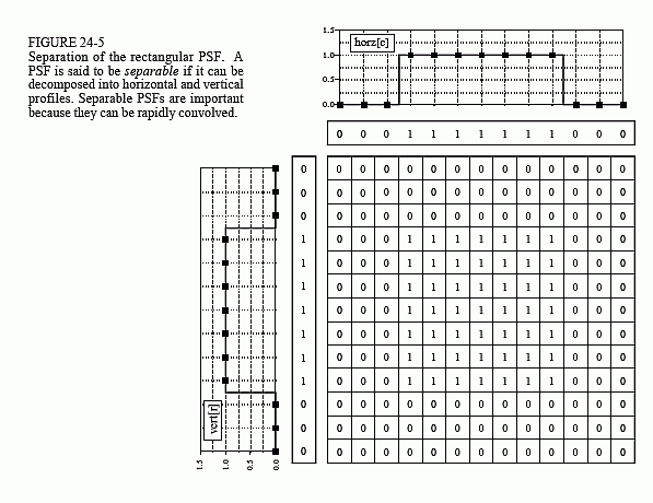
This is a technique for fast convolution, as long as the PSF is separable. A PSF is said to be separable if it can be broken into two one-dimensional signals: a vertical and a horizontal projection. Figure 24-5 shows an example of a separable image, the square PSF. Specifically, the value of each pixel in the image is equal to the corresponding point in the horizontal projection multiplied by the corresponding point in the vertical projection. In mathematical form:

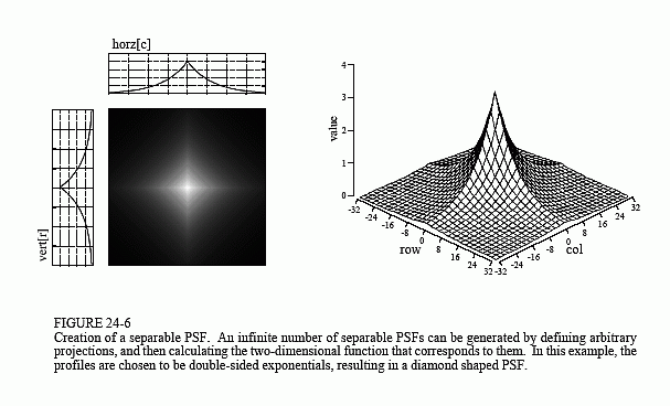
where x[r,c] is the two-dimensional image, and vert[r] & horz[c] are the one-dimensional projections. Obviously, most images do not satisfy this requirement. For example, the pillbox is not separable. There are, however, an infinite number of separable images. This can be understood by generating arbitrary horizontal and vertical projections, and finding the image that corresponds to them. For example, Fig. 24-6 illustrates this with profiles that are double-sided exponentials. The image that corresponds to these profiles is then found from Eq. 24-1. When displayed, the image appears as a diamond shape that exponentially decays to zero as the distance from the origin increases.

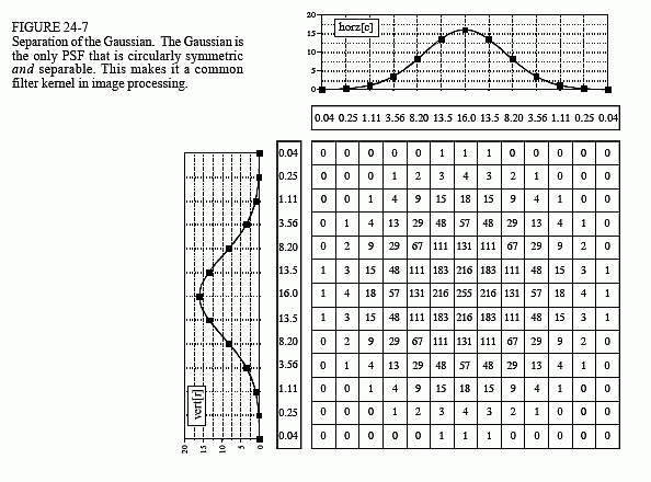
In most image processing tasks, the ideal PSF is circularly symmetric, such as the pillbox. Even though digitized images are usually stored and processed in the rectangular format of rows and columns, it is desired to modify the image the same in all directions. This raises the question: is there a PSF that is circularly symmetric and separable? The answer is, yes,

but there is only one, the Gaussian. As is shown in Fig. 24-7, a two-dimensional Gaussian image has projections that are also Gaussians. The image and projection Gaussians have the same standard deviation.

To convolve an image with a separable filter kernel, convolve each row in the image with the horizontal projection, resulting in an intermediate image. Next, convolve each column of this intermediate image with the vertical projection of the PSF. The resulting image is identical to the direct convolution of the original image and the filter kernel. If you like, convolve the columns first and then the rows; the result is the same.

The convolution of an N×N image with an M×M filter kernel requires a time proportional to N²M². In other words, each pixel in the output image depends on all the pixels in the filter kernel. In comparison, convolution by separability only requires a time proportional to N²M. For filter kernels that are hundreds of pixels wide, this technique will reduce the execution time by a factor of hundreds.

Things can get even better. If you are willing to use a rectangular PSF (Fig. 24-5) or a double-sided exponential PSF (Fig. 24-6), the calculations are even more efficient. This is because the one-dimensional convolutions are the moving average filter (Chapter 15) and the bidirectional single pole filter (Chapter 19), respectively. Both of these one-dimensional filters can be rapidly carried out by recursion. This results in an image convolution time proportional to only N², completely independent of the size of the PSF. In other words, an image can be convolved with as large a PSF as needed, with only a few integer operations per pixel. For example, the convolution of a 512×512 image requires only a few hundred milliseconds on a personal computer. That's fast! Don't like the shape of these two filter kernels? Convolve the image with one of them several times to approximate a Gaussian PSF (guaranteed by the Central Limit Theorem, Chapter 7). These are great algorithms, capable of snatching success from the jaws of failure. They are well worth remembering.