The Scientist and Engineer's Guide to
Digital Signal Processing
By Steven W. Smith, Ph.D.

• Home
• The Book by Chapters
• About the Book
  • Copyright and permissible use
  • What is DSP?
  • 8 good reasons for learning DSP
  • Comments by reviewers
  • Errata
  • Free Software and Teaching Aids
  • Differences Between Editions
• Steven W. Smith
• Blog
• Contact

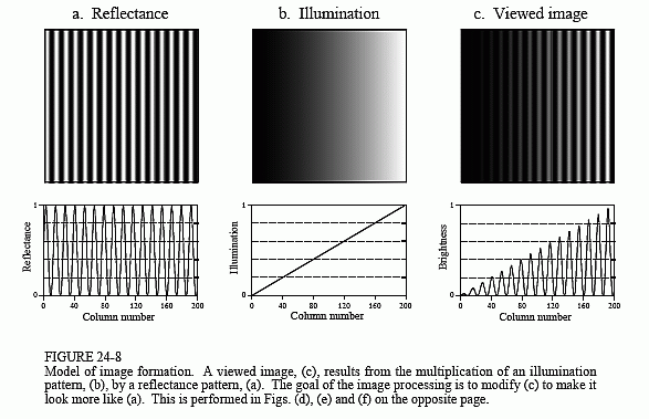
A common application requiring a large PSF is the enhancement of images with unequal illumination. Convolution by separability is an ideal algorithm to carry out this processing. With only a few exceptions, the images seen by the eye are formed from reflected light. This means that a viewed image is equal to the reflectance of the objects multiplied by the ambient illumination. Figure 24-8 shows how this works. Figure (a) represents the reflectance of a scene being viewed, in this case, a series of light and dark bands. Figure (b) illustrates an example illumination signal, the pattern of light falling on (a). As in the real world, the illumination slowly varies over the imaging area. Figure (c) is the image seen by the eye, equal to the reflectance image, (a), multiplied by the illumination image, (b). The regions of poor illumination are difficult to view in (c) for two reasons: they are too dark and their contrast is too low (the difference between the peaks and the valleys).

To understand how this relates to the problem of every day vision, imagine you are looking at two identically dressed men. One of them is standing in the bright sunlight, while the other is standing in the shade of a nearby tree. The percent of the incident light reflected from both men is the same. For instance, their faces might reflect 80% of the incident light, their gray shirts 40% and their dark pants 5%. The problem is, the illumination of the two might be, say, ten times different. This makes the image of the man in the shade ten times darker than the person in the sunlight, and the contrast (between the face, shirt, and pants) ten times less.

The goal of the image processing is to flatten the illumination component in the acquired image. In other words, we want the final image to be representative of the objects' reflectance, not the lighting conditions. In terms of Fig. 24-8, given (c), find (a). This is a nonlinear filtering problem, since the component images were combined by multiplication, not addition. While this separation cannot be performed perfectly, the improvement can be dramatic.

To start, we will convolve image (c) with a large PSF, one-fifth the size of the entire image. The goal is to eliminate the sharp features in (c), resulting

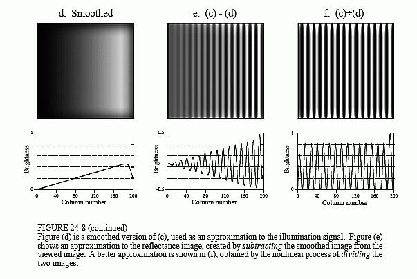
in an approximation to the original illumination signal, (b). This is where convolution by separability is used. The exact shape of the PSF is not important, only that it is much wider than the features in the reflectance image. Figure (d) is the result, using a Gaussian filter kernel.

Since a smoothing filter provides an estimate of the illumination image, we will use an edge enhancement filter to find the reflectance image. That is, image (c) will be convolved with a filter kernel consisting of a delta function minus a Gaussian. To reduce execution time, this is done by subtracting the smoothed image in (d) from the original image in (c). Figure (e) shows the result. It doesn't work! While the dark areas have been properly lightened, the contrast in these areas is still terrible.

Linear filtering performs poorly in this application because the reflectance and illumination signals were original combined by multiplication, not addition. Linear filtering cannot correctly separate signals combined by a nonlinear operation. To separate these signals, they must be unmultiplied. In other words, the original image should be divided by the smoothed image, as is shown in (f). This corrects the brightness and restores the contrast to the proper level.

This procedure of dividing the images is closely related to homomorphic processing, previously described in Chapter 22. Homomorphic processing is a way of handling signals combined through a nonlinear operation. The strategy is to change the nonlinear problem into a linear one, through an appropriate mathematical operation. When two signals are combined by

multiplication, homomorphic processing starts by taking the logarithm of the acquired signal. With the identity: log(a×b) = log(a) + log(b), the problem of separating multiplied signals is converted into the problem of separating added signals. For example, after taking the logarithm of the image in (c), a linear high-pass filter can be used to isolate the logarithm of the reflectance image. As before, the quickest way to carry out the high-pass filter is to subtract a smoothed version of the image. The antilogarithm (exponent) is then used to undo the logarithm, resulting in the desired approximation to the reflectance image.

Which is better, dividing or going along the homomorphic path? They are nearly the same, since taking the logarithm and subtracting is equal to dividing. The only difference is the approximation used for the illumination image. One method uses a smoothed version of the acquired image, while the other uses a smoothed version of the logarithm of the acquired image.

This technique of flattening the illumination signal is so useful it has been incorporated into the neural structure of the eye. The processing in the middle layer of the retina was previously described as an edge enhancement or high-pass filter. While this is true, it doesn't tell the whole story. The first layer of the eye is nonlinear, approximately taking the logarithm of the incoming image. This makes the eye a homomorphic processor. Just as described above, the logarithm followed by a linear edge enhancement filter flattens the illumination component, allowing the eye to see under poor lighting conditions. Another interesting use of homomorphic processing occurs in photography. The density (darkness) of a negative is equal to the logarithm of the brightness in the final photograph. This means that any manipulation of the negative during the development stage is a type of homomorphic processing.

Before leaving this example, there is a nuisance that needs to be mentioned.

As discussed in Chapter 6, when an N point signal is convolved with an M point filter kernel, the resulting signal is N+M-1 points long. Likewise, when an M×M image is convolved with an N×N filter kernel, the result is an (M+N-1) × (M+N-1) image. The problem is, it is often difficult to manage a changing image size. For instance, the allocated memory must change, the video display must be adjusted, the array indexing may need altering, etc. The common way around this is to ignore it; if we start with a 512×512 image, we want to end up with a 512×512 image. The pixels that do not fit within the original boundaries are discarded.

While this keeps the image size the same, it doesn't solve the whole problem; these is still the boundary condition for convolution. For example, imagine trying to calculate the pixel at the upper-right corner of (d). This is done by centering the Gaussian PSF on the upper-right corner of (c). Each pixel in (c) is then multiplied by the corresponding pixel in the overlaying PSF, and the products are added. The problem is, three-quarters of the PSF lies outside the defined image. The easiest approach is to assign the undefined pixels a value of zero. This is how (d) was created, accounting for the dark band around the perimeter of the image. That is, the brightness smoothly decreases to the pixel value of zero, exterior to the defined image.

Fortunately, this dark region around the boarder can be corrected (although it hasn't been in this example). This is done by dividing each pixel in (d) by a correction factor. The correction factor is the fraction of the PSF that was immersed in the input image when the pixel was calculated. That is, to correct an individual pixel in (d), imagine that the PSF is centered on the corresponding pixel in (c). For example, the upper-right pixel in (c) results from only 25% of the PSF overlapping the input image. Therefore, correct this pixel in (d) by dividing it by a factor of 0.25. This means that the pixels in the center of (d) will not be changed, but the dark pixels around the perimeter will be brightened. To find the correction factors, imagine convolving the filter kernel with an image having all the pixel values equal to one. The pixels in the resulting image are the correction factors needed to eliminate the edge effect.