The Scientist and Engineer's Guide to
Digital Signal Processing
By Steven W. Smith, Ph.D.

• Home
• The Book by Chapters
• About the Book
  • Copyright and permissible use
  • What is DSP?
  • 8 good reasons for learning DSP
  • Comments by reviewers
  • Errata
  • Free Software and Teaching Aids
  • Differences Between Editions
• Steven W. Smith
• Blog
• Contact

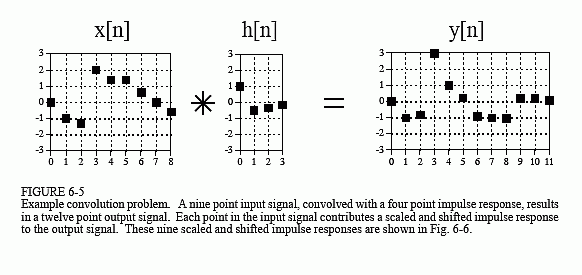
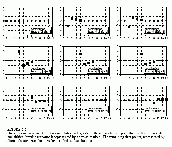
Figure 6-5 shows a simple convolution problem: a 9 point input signal, x[n], is passed through a system with a 4 point impulse response, h[n], resulting in a 9 + 4 - 1 = 12 point output signal, y[n]. In mathematical terms, x[n] is convolved with h[n] to produce y[n]. This first viewpoint of convolution is based on the fundamental concept of DSP: decompose the input, pass the components through the system, and synthesize the output. In this example, each of the nine samples in the input signal will contribute a scaled and shifted version of the impulse response to the output signal. These nine signals are shown in Fig. 6-6. Adding these nine signals produces the output signal, y[n].

Let's look at several of these nine signals in detail. We will start with sample number four in the input signal, i.e., x[4]. This sample is at index number four, and has a value of 1.4. When the signal is decomposed, this turns into an impulse represented as: 1.4δ[n-4]. After passing through the system, the resulting output component will be: 1.4h[n-4]. This signal is shown in the center box of the nine signals in Fig. 6-6. Notice that this is the impulse response, h[n], multiplied by 1.4, and shifted four samples to the right. Zeros have been added at samples 0-3 and at samples 8-11 to serve as place holders. To make this more clear, Fig. 6-6 uses squares to represent the data points that come from the shifted and scaled impulse response, and diamonds for the added zeros.

Now examine sample x[8], the last point in the input signal. This sample is at index number eight, and has a value of -0.5. As shown in the lower-right graph of Fig. 6-6, x[8] results in an impulse response that has been shifted to the right by eight points and multiplied by -0.5. Place holding zeros have been added at points 0-7. Lastly, examine the effect of points x[0] and x[7]. Both these samples have a value of zero, and therefore produce output components consisting of all zeros.

In this example, is a nine point signal and is a four point signal. In our next example, shown in Fig. 6-7, we will reverse the situation by making a four point signal, and a nine point signal. The same two waveforms are used, they are just swapped. As shown by the output signal components, the four samples in result in four shifted and scaled versions of the nine point impulse response. Just as before, leading and trailing zeros are added as place holders.

But wait just one moment! The output signal in Fig. 6-7 is identical to the output signal in Fig. 6-5. This isn't a mistake, but an important property. Convolution is commutative: a[n]*b[n] = b[n]*a[n]. The mathematics does not care which is the input signal and which is the impulse response, only that two signals are convolved with each other. Although the mathematics may allow it, exchanging the two signals has no physical meaning in system theory. The input signal and impulse response are two totally different things and exchanging them doesn't make sense. What the commutative property provides is a mathematical tool for manipulating equations to achieve various results.

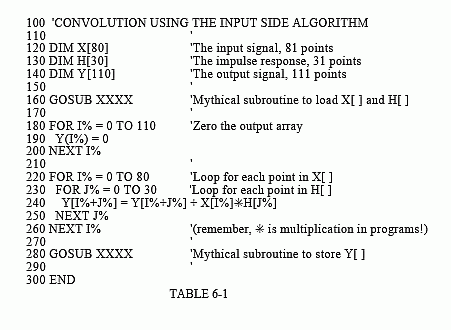
A program for calculating convolutions using the input side algorithm is shown in Table 6-1. Remember, the programs in this book are meant to convey algorithms in the simplest form, even at the expense of good programming style. For instance, all of the input and output is handled in mythical subroutines (lines 160 and 280), meaning we do not define how these operations are conducted. Do not skip over these programs; they are a key part of the material and you need to understand them in detail.

The program convolves an 81 point input signal, held in array X[ ], with a 31 point impulse response, held in array H[ ], resulting in a 111 point output signal, held in array Y[ ]. These are the same lengths shown in Figs. 6-3 and 6-4. Notice that the names of these arrays use upper case letters. This is a violation of the naming conventions previously discussed, because upper case letters are reserved for frequency domain signals. Unfortunately, the simple BASIC used in this book does not allow lower case variable names. Also notice that line 240 uses a star for multiplication. Remember, a star in a program means multiplication, while a star in an equation means convolution. A star in text (such as documentation or program comments) can mean either.

The mythical subroutine in line 160 places the input signal into X[ ] and the impulse response into H[ ]. Lines 180-200 set all of the values in Y[ ] to zero. This is necessary because Y[ ] is used as an accumulator to sum the output components as they are calculated. Lines 220 to 260 are the heart of the program. The FOR statement in line 220 controls a loop that steps through each point in the input signal, X[ ]. For each sample in the input signal, an inner loop (lines 230-250) calculates a scaled and shifted version of the impulse response, and adds it to the array accumulating the output signal, Y[ ]. This nested loop structure (one loop within another loop) is a key characteristic of convolution programs; become familiar with it.

Keeping the indexing straight in line 240 can drive you crazy! Let's say we are halfway through the execution of this program, so that we have just begun action on sample X[40], i.e., I% = 40. The inner loop runs through each point in the impulse response doing three things. First, the impulse response is scaled by multiplying it by the value of the input sample. If this were the only action taken by the inner loop, line 240 could be written, Y[J%] = X[40]✳H[J%]. Second, the scaled impulse is shifted 40 samples to the right by adding this number to the index used in the output signal. This second action would change line 240 to: Y[40+J%] = X[40]*H[J%]. Third, Y[ ] must accumulate (synthesize) all the signals resulting from each sample in the input signal. Therefore, the new information must be added to the information that is already in the array. This results in the final command: Y[40+J%] = Y[40+J%] + X[40]*H[J%]. Study this carefully; it is very confusing, but very important.