The Scientist and Engineer's Guide to
Digital Signal Processing
By Steven W. Smith, Ph.D.

• Home
• The Book by Chapters
• About the Book
  • Copyright and permissible use
  • What is DSP?
  • 8 good reasons for learning DSP
  • Comments by reviewers
  • Errata
  • Free Software and Teaching Aids
  • Differences Between Editions
• Steven W. Smith
• Blog
• Contact

The first viewpoint of convolution analyzes how each sample in the input signal affects many samples in the output signal. In this second viewpoint, we reverse this by looking at individual samples in the output signal, and finding the contributing points from the input. This is important from both mathematical and practical standpoints. Suppose that we are given some input signal and impulse response, and want to find the convolution of the two. The most straightforward method would be to write a program that loops through the output signal, calculating one sample on each loop cycle. Likewise, equations are written in the form: y[n] = some combination of other variables. That is, sample n in the output signal is equal to some combination of the many values in the input signal and impulse response. This requires a knowledge of how each sample in the output signal can be calculated independently of all other samples in the output signal. The output side algorithm provides this information.

Let's look an example of how a single point in the output signal is influenced by several points from the input. The example point we will use is y[6] in Fig. 6-5. This point is equal to the sum of all the sixth points in the nine output components, shown in Fig. 6-6. Now, look closely at these nine output components and identify which can affect y[6]. That is, find which of these nine signals contains a nonzero sample at the sixth position. Five of the output components only have added zeros (the diamond markers) at the sixth sample, and can therefore be ignored. Only four of the output components are capable of having a nonzero value in the sixth position. These are the output components generated from the input samples: x[3], x[4], x[5] and x[6]. By adding the sixth sample from each of these output components, y[6] is determined as: y[6] = x[3]h[3] + x[4]h[2] + x[5]h[1] + x[6]h[0]. That is, four samples from the input signal are multiplied by the four samples in the impulse response, and the products added.

Figure 6-8 illustrates the output side algorithm as a convolution machine, a flow diagram of how convolution occurs. Think of the input signal, x[n], and the output signal, y[n], as fixed on the page. The convolution machine, everything inside the dashed box, is free to move left and right as needed. The convolution machine is positioned so that its output is aligned with the output sample being calculated. Four samples from the input signal fall into the inputs of the convolution machine. These values are multiplied by the indicated samples in the impulse response, and the products are added. This produces the value for the output signal, which drops into its proper place. For example, y[n] is shown being calculated from the four input samples: x[3], x[4], x[5], and x[6].

To calculate y[7], the convolution machine moves one sample to the right. This results in another four samples entering the machine, x[4] through x[7], and the value for y[7] dropping into the proper place. This process is repeated for all points in the output signal needing to be calculated.

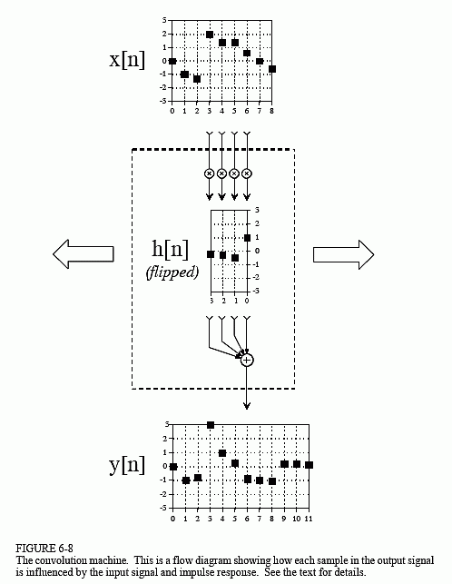
The arrangement of the impulse response inside the convolution machine is very important. The impulse response is flipped left-for-right. This places sample number zero on the right, and increasingly positive sample numbers running to the left. Compare this to the normal impulse response in Fig. 6-5 to understand the geometry of this flip. Why is this flip needed? It simply falls out of the mathematics. The impulse response describes how each point in the input signal affects the output signal. This results in each point in the output signal being affected by points in the input signal weighted by a flipped impulse response.

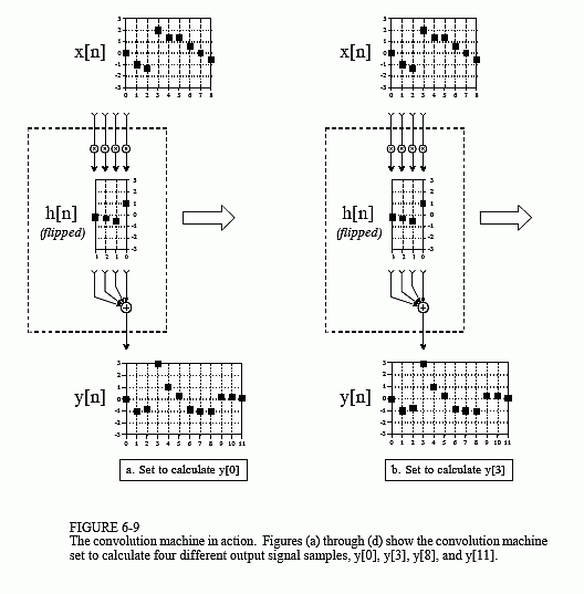
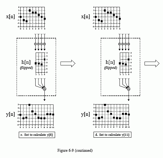
Figure 6-9 shows the convolution machine being used to calculate several samples in the output signal. This diagram also illustrates a real nuisance in convolution. In (a), the convolution machine is located fully to the left with its output aimed at . In this position, it is trying to receive input from samples: x[-3], x[-2], x[-1] and x[0]. The problem is, three of these samples: x[-3], x[-2] and x[-1] do not exist! This same dilemma arises in (d), where the convolution machine tries to accept samples to the right of the defined input signal, points x[9], x[10] and x[11].

One way to handle this problem is by inventing the nonexistent samples. This involves adding samples to the ends of the input signal, with each of the added samples having a value of zero. This is called padding the signal with zeros. Instead of trying to access a nonexistent value, the convolution machine receives a sample that has a value of zero. Since this zero is eliminated during the multiplication, the result is mathematically the same as ignoring the nonexistent inputs.

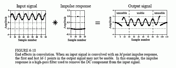
The important part is that the far left and far right samples in the output signal are based on incomplete information. In DSP jargon, the impulse response is not fully immersed in the input signal. If the impulse response is M points in length, the first and last M-1 samples in the output signal are based on less information than the samples between. This is analogous to an electronic circuit requiring a certain amount of time to stabilize after the power is applied. The difference is that this transient is easy to ignore in electronics, but very prominent in DSP.

Figure 6-10 shows an example of the trouble these end effects can cause. The input signal is a sine wave plus a DC component. The desire is to remove the DC part of the signal, while leaving the sine wave intact. This calls for a high-pass filter, such as the impulse response shown in the figure. The problem is, the first and last 30 points are a mess! The shape of these end regions can be understood by imagining the input signal padded with 30 zeros on the left side, samples x[-1] through x[-30], and 30 zeros on the right, samples x[81] through x[110]. The output signal can then be viewed as a filtered version of this longer waveform. These "end effect" problems are widespread in DSP. As a general rule, expect that the beginning and ending samples in processed signals will be quite useless.

Now the math. Using the convolution machine as a guideline, we can write the standard equation for convolution. If x[n] is an N point signal running from 0 to N-1, and h[n] is an M point signal running from 0 to M-1, the convolution of the two: y[n] = x[n] * h[n], is an N+M-1 point signal running from 0 to N+M-2, given by:

This equation is called the convolution sum. It allows each point in the output signal to be calculated independently of all other points in the output signal. The index, i, determines which sample in the output signal is being calculated, and therefore corresponds to the left-right position of the convolution machine. In computer programs performing convolution, a loop makes this index run through each sample in the output signal. To calculate one of the output samples, the index, j, is used inside of the convolution machine. As j runs through 0 to M-1, each sample in the impulse response, h[j], is multiplied by the proper sample from the input signal, x[i-j]. All these products are added to produce the output sample being calculated. Study Eq. 6-1 until you fully understand how it is implemented by the convolution machine. Much of DSP is based on this equation. (Don't be confused by the n in y[n] = x[n] * h[n]. This is merely a place holder to indicate that some variable is the index into the array. Sometimes the equations are written: y[] = x[] * h[], just to avoid having to bring in a meaningless symbol).

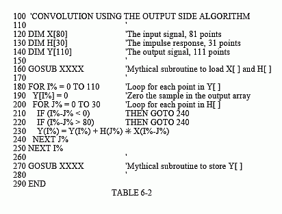
Table 6-2 shows a program for performing convolutions using the output side algorithm, a direct use of Eq. 6-1. This program produces the same output signal as the program for the input side algorithm, shown previously in Table 6-1. Notice the main difference between these two programs: the input side algorithm loops through each sample in the input signal (line 220 of Table 6-1), while the output side algorithm loops through each sample in the output signal (line 180 of Table 6-2).

Here is a detailed operation of this program. The FOR-NEXT loop in lines 180 to 250 steps through each sample in the output signal, using I% as the index. For each of these values, an inner loop, composed of lines 200 to 230, calculates the value of the output sample, Y[I%]. The value of Y[I%] is set to zero in line 190, allowing it to accumulate the products inside of the convolution machine. The FOR-NEXT loop in lines 200 to 240 provide a direct implementation of Eq. 6-2. The index, J%, steps through each

sample in the impulse response. Line 230 provides the multiplication of each sample in the impulse response, H[J%], with the appropriate sample from the input signal, X[I%-J%], and adds the result to the accumulator.

In line 230, the sample taken from the input signal is: X[I%-J%]. Lines 210 and 220 prevent this from being outside the defined array, X[0] to X[80]. In other words, this program handles undefined samples in the input signal by ignoring them. Another alternative would be to define the input signal's array from X[-30] to X[110], allowing 30 zeros to be padded on each side of the true data. As a third alternative, the FOR-NEXT loop in line 180 could be changed to run from 30 to 80, rather than 0 to 110. That is, the program would only calculate the samples in the output signal where the impulse response is fully immersed in the input signal. The important thing is that you must use one of these three techniques. If you don't, the program will crash when it tries to read the out-of-bounds data.