The Scientist and Engineer's Guide to
Digital Signal Processing
By Steven W. Smith, Ph.D.

• Home
• The Book by Chapters
• About the Book
  • Copyright and permissible use
  • What is DSP?
  • 8 good reasons for learning DSP
  • Comments by reviewers
  • Errata
  • Free Software and Teaching Aids
  • Differences Between Editions
• Steven W. Smith
• Blog
• Contact

Commutative Property
The commutative property for convolution is expressed in mathematical form:

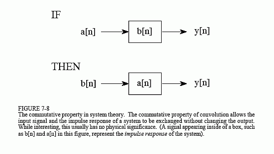
In words, the order in which two signals are convolved makes no difference; the results are identical. As shown in Fig. 7-8, this has a strange meaning for system theory. In any linear system, the input signal and the system's impulse response can be exchanged without changing the output signal. This is interesting, but usually doesn't have any physical meaning. The input signal and the impulse response are very different things. Just because the mathematics allows you to do something, doesn't mean that it makes sense to do it. For example, suppose you make: $10/hour ? 2,000 hours/year = $20,000/year. The commutative property for multiplication provides that you can make the same annual salary by only working 10 hours/year at $2000/hour. Let's see you convince your boss that this is meaningful! In spite of this, the commutative property sees great use in DSP for manipulating equations, just as in ordinary algebra.

Associative Property
Is it possible to convolve three or more signals? The answer is yes, and the associative property describes how: convolve two of the signals to produce an intermediate signal, then convolve the intermediate signal with the third signal. The associative property provides that the order of the convolutions doesn't matter. As an equation:

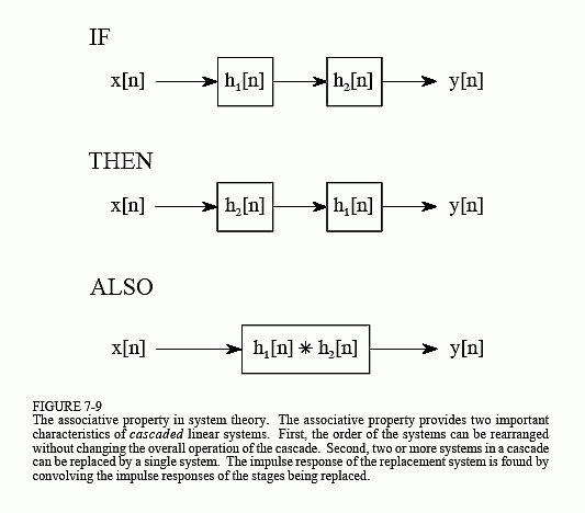
The associative property is used in system theory to describe how cascaded systems behave. As shown in Fig. 7-9, two or more systems are said to be in a cascade if the output of one system is used as the input for the next system. From the associative property, the order of the systems can be rearranged without changing the overall response of the cascade. Further, any number of cascaded systems can be replaced with a single system. The impulse response of the replacement system is found by convolving the impulse responses of all of the original systems.

Distributive Property
In equation form, the distributive property is written:

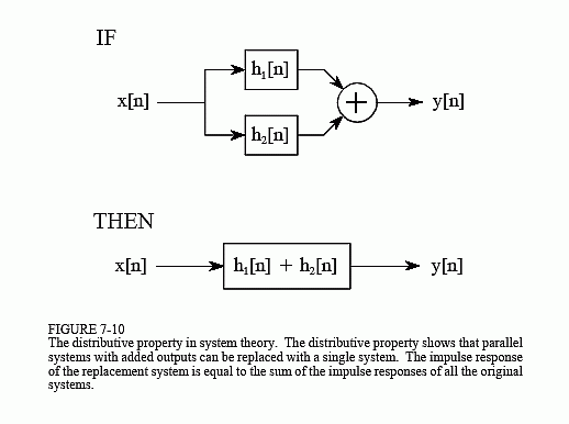
The distributive property describes the operation of parallel systems with added outputs. As shown in Fig. 7-10, two or more systems can share the same input, x[n], and have their outputs added to produce y[n]. The distributive property allows this combination of systems to be replaced with a single system, having an impulse response equal to the sum of the impulse responses of the original systems.

Transference between the Input and Output
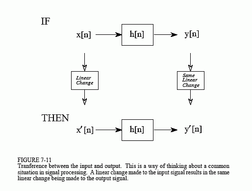
Rather than being a formal mathematical property, this is a way of thinking about a common situation in signal processing. As illustrated in Fig. 7-11, imagine a linear system receiving an input signal, x[n], and generating an output signal, y[n]. Now suppose that the input signal is changed in some linear way, resulting in a new input signal, which we will call x´[n]. This results in a new output signal, y?[n]. The question is, how does the change in the input signal relate to the change in the output signal? The answer is: the output signal is changed in exactly the same linear way that the input signal was changed. For example, if the input signal is amplified by a factor of two, the output signal will also be amplified by a factor of two. If the derivative is taken of the input signal, the derivative will also be taken of the output signal. If the input is filtered in some way, the output will be filtered in an identical manner. This can easily be proven by using the associative property.

The Central Limit Theorem
The Central Limit Theorem is an important tool in probability theory because it mathematically explains why the Gaussian probability distribution is observed so commonly in nature. For example: the amplitude of thermal noise in electronic circuits follows a Gaussian distribution; the cross-sectional intensity of a laser beam is Gaussian; even the pattern of holes around a dart board bull's eye is Gaussian. In its simplest form, the Central Limit Theorem states that a Gaussian distribution results when the observed variable is the sum of many random processes. Even if the component processes do not have a Gaussian distribution, the sum of them will.

The Central Limit Theorem has an interesting implication for convolution. If a pulse-like signal is convolved with itself many times, a Gaussian is produced. Figure 7-12 shows an example of this. The signal in (a) is an

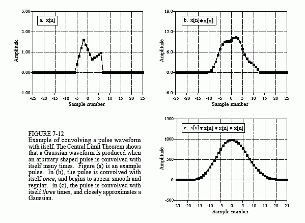
irregular pulse, purposely chosen to be very unlike a Gaussian. Figure (b) shows the result of convolving this signal with itself one time. Figure (c) shows the result of convolving this signal with itself three times. Even with only three convolutions, the waveform looks very much like a Gaussian. In mathematics jargon, the procedure converges to a Gaussian very quickly. The width of the resulting Gaussian (i.e., σ in Eq. 2-7 or 2-8) is equal to the width of the original pulse (expressed as σ in Eq. 2-7) multiplied by the square root of the number of convolutions.