The Scientist and Engineer's Guide to
Digital Signal Processing
By Steven W. Smith, Ph.D.

• Home
• The Book by Chapters
• About the Book
  • Copyright and permissible use
  • What is DSP?
  • 8 good reasons for learning DSP
  • Comments by reviewers
  • Errata
  • Free Software and Teaching Aids
  • Differences Between Editions
• Steven W. Smith
• Blog
• Contact

The DFT can be calculated in three completely different ways. First, the problem can be approached as a set of simultaneous equations. This method is useful for understanding the DFT, but it is too inefficient to be of practical use. The second method brings in an idea from the last chapter: correlation. This is based on detecting a known waveform in another signal. The third method, called the Fast Fourier Transform (FFT), is an ingenious algorithm that decomposes a DFT with N points, into N DFTs each with a single point. The FFT is typically hundreds of times faster than the other methods. The first two methods are discussed here, while the FFT is the topic of Chapter 12. It is important to remember that all three of these methods produce an identical output. Which should you use? In actual practice, correlation is the preferred technique if the DFT has less than about 32 points, otherwise the FFT is used.

DFT by Simultaneous Equations
Think about the DFT calculation in the following way. You are given N values from the time domain, and asked to calculate the N values of the frequency domain (ignoring the two frequency domain values that you know must be zero). Basic algebra provides the answer: to solve for N unknowns, you must be able to write N linearly independent equations. To do this, take the first sample from each sinusoid and add them together. The sum must be equal to the first sample in the time domain signal, thus providing the first equation. Likewise, an equation can be written for each of the remaining points in the time domain signal, resulting in the required N equations. The solution can then be found by using established methods for solving simultaneous equations, such as Gauss Elimination. Unfortunately, this method requires a tremendous number of calculations, and is virtually never used in DSP. However, it is important for another reason, it shows why it is possible to decompose a signal into sinusoids, how many sinusoids are needed, and that the basis functions must be linearly independent (more about this shortly).

DFT by Correlation
Let's move on to a better way, the standard way of calculating the DFT. An example will show how this method works. Suppose we are trying to calculate the DFT of a 64 point signal. This means we need to calculate the 33 points in the real part, and the 33 points in the imaginary part of the frequency domain. In this example we will only show how to calculate a single sample, ImX[3], i.e., the amplitude of the sine wave that makes three complete cycles between point 0 and point 63. All of the other frequency domain values are calculated in a similar manner.

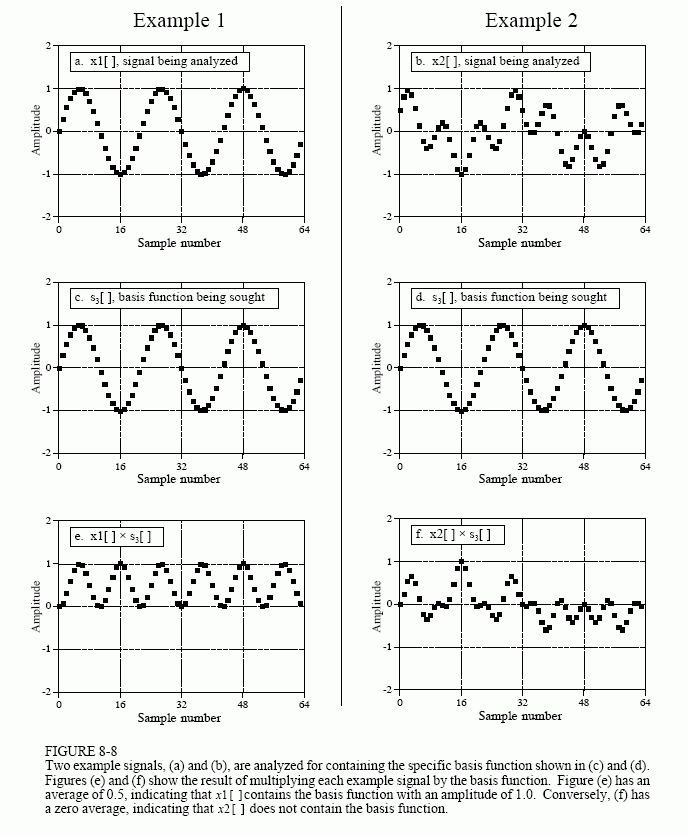
Figure 8-8 illustrates using correlation to calculate ImX[3]. Figures (a) and (b) show two example time domain signals, called: x1[ ] and x2[ ], respectively. The first signal, x1[ ], is composed of nothing but a sine wave that makes three cycles between points 0 and 63. In contrast, x2[ ] is composed of several sine and cosine waves, none of which make three cycles between points 0 and 63. These two signals illustrate what the algorithm for calculating ImX[3] must do. When fed x1[ ], the algorithm must produce a value of 32, the amplitude of the sine wave present in the signal (modified by the scaling factors of Eq. 8-3). In comparison, when the algorithm is fed the other signal, x2[ ], a value of zero must be produced, indicating that this particular sine wave is not present in this signal.

The concept of correlation was introduced in Chapter 7. Briefly, to detect a known waveform contained in another signal, multiply the two and add the points in the resulting product. The single number that results from this procedure is a measure of how similar the two signals are. Figure 8-8 illustrates this approach. Figures (c) and (d) both display the signal we are looking for, a sine wave that makes 3 cycles between samples 0 and 63. Figure (e) shows the result of multiplying (a) and (c). Likewise, (f) shows the result of multiplying (b) and (d). The sum of all the points in (e) is 32, while the sum of all the points in (f) is zero, showing we have found the desired algorithm.

The other samples in the frequency domain are calculated in the same way. This procedure is formalized in the analysis equation, the mathematical way to calculate the frequency domain from the time domain:

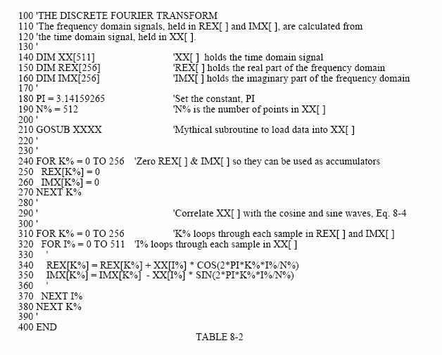
In words, each sample in the frequency domain is found by multiplying the time domain signal by the sine or cosine wave being looked for, and adding the resulting points. If someone asks you what you are doing, say with confidence: "I am correlating the input signal with each basis function." Table 8-2 shows a computer program for calculating the DFT in this way.

The analysis equation does not require special handling of the first and last points, as did the synthesis equation. There is, however, a negative sign in the imaginary part in Eq. 8-4. Just as before, this negative sign makes the real DFT consistent with the complex DFT, and is not always included.

In order for this correlation algorithm to work, the basis functions must have an interesting property: each of them must be completely uncorrelated with all of the others. This means that if you multiply any two of the basis functions, the sum of the resulting points will be equal to zero. Basis functions that have this property are called orthognal. Many other

orthognal basis functions exist, including: square waves, triangle waves, impulses, etc. Signals can be decomposed into these other orthognal basis functions using correlation, just as done here with sinusoids. This is not to suggest that this is useful, only that it is possible.

As previously shown in Table 8-1, the Inverse DFT has two ways to be implemented in a computer program. This difference involves swapping the inner and outer loops during the synthesis. While this does not change the output of the program, it makes a difference in how you view what is being done. The DFT program in Table 8-2 can also be changed in this fashion, by swapping the inner and outer loops in lines 310 to 380. Just as before, the output of the program is the same, but the way you think about the calculation is different. (These two different ways of viewing the DFT and inverse DFT could be described as "input side" and "output side" algorithms, just as for convolution).

As the program in Table 8-2 is written, it describes how an individual sample in the frequency domain is affected by all of the samples in the time domain. That is, the program calculates each of the values in the frequency domain in succession, not as a group. When the inner and outer loops are exchanged, the program loops through each sample in the time domain, calculating the contribution of that point to the frequency domain. The overall frequency domain is found by adding the contributions from the individual time domain points. This brings up our next question: what kind of contribution does an individual sample in the time domain provide to the frequency domain? The answer is contained in an interesting aspect of the Fourier domain called duality.